Pivoting Data Columns Into Rows
Some data files may contain repeating columns, such as sales figures for a series of years. There may even be repeating column groups, such as both budget and actual figures for a series of years.
When a data source includes multiple measure columns that provide values for the same type of measurement, it may be useful to pivot these columns into rows. This results in a simpler table with fewer columns, and with more dimension fields for sorting your data.
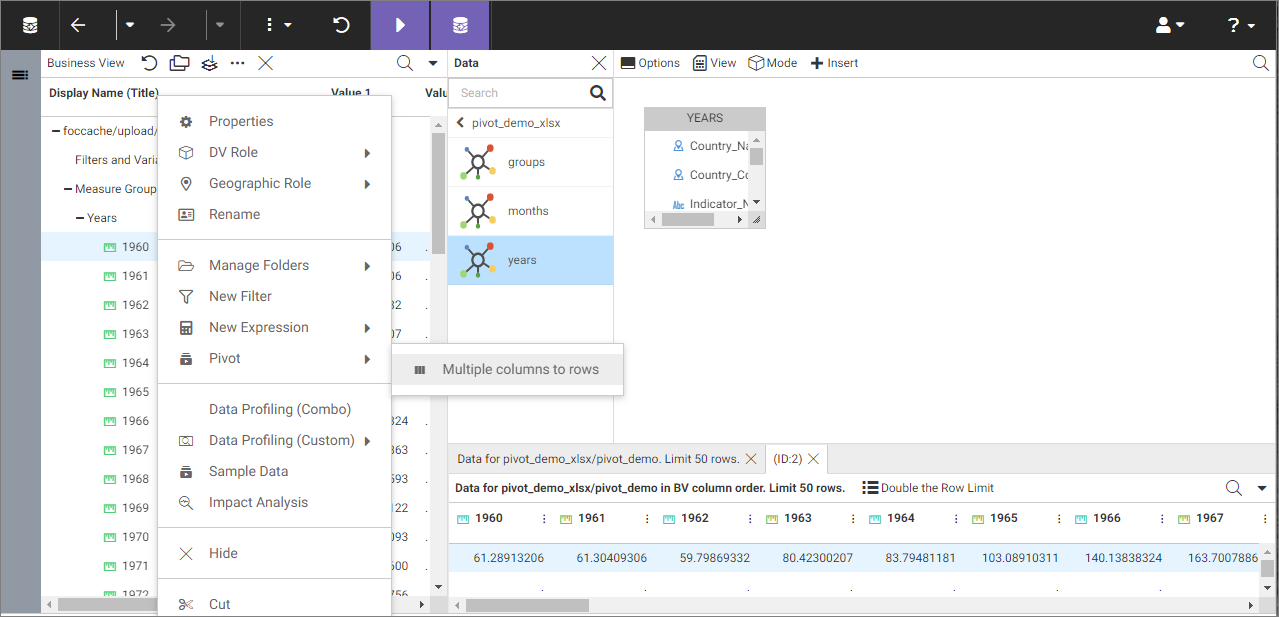
When uploading data, you can use the pivot option to transform these columns or groups of columns into rows, as shown in the following image.
Note: The pivot option is also available when creating or editing metadata.
Pivot Columns Into Rows
- Right-click a field name in the Business View panel, point to Pivot, and then click Multiple columns to rows. The Pivot Columns to Rows dialog box opens.
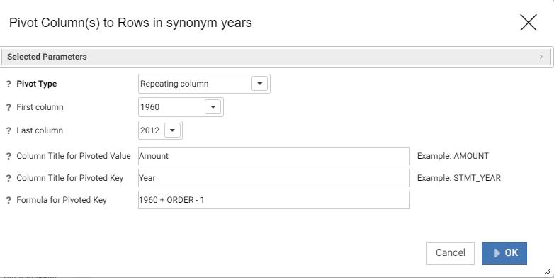
- In the Pivot Type drop-down menu, select Repeating column. This is the default setting.
- In the First column drop-down menu, select the first column in the range of repeating columns.
- In the Last column drop-down menu, select the last column in the range of repeating columns.
- In the Column Title for Pivoted Value, type the new column title that reflects the numeric field that you are creating.
- In the Column Title for Pivoted Key field, which will be a new dimension field, type the new column title that represents the repeating columns that you are pivoting into rows.
- Leave the Formula for Pivoted Key field value unedited. This value is automatically generated and should not be changed. An example of the completed configuration for pivoting columns is shown in the following image.
- Click OK
Note: To revert your pivoting changes, right-click the synonym on the Join Editor canvas, and click Remove Pivot.
Pivot Column Groups into Rows
1. Right-click a field name in the Business View panel, point to Pivot, and then click Multiple columns to rows.
The Pivot Columns to Rows dialog box opens.
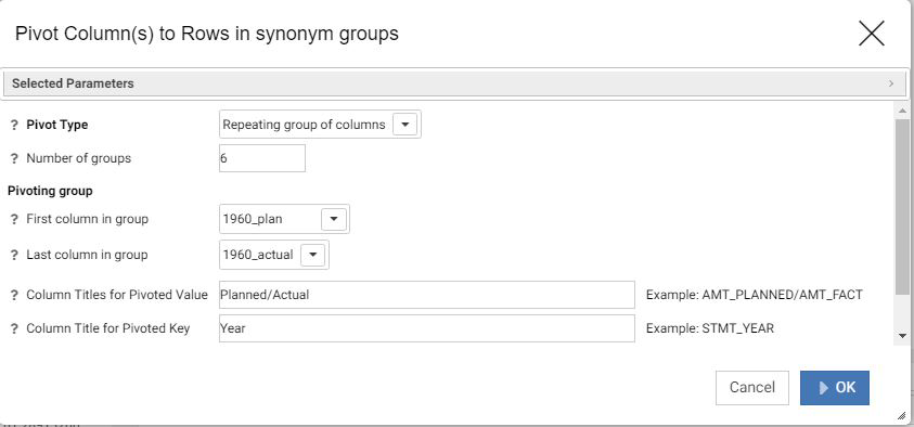
2. In the Pivot Type drop-down menu, select Repeating group of columns.
3. In the Number of groups field, specify the number of groups of columns that you are pivoting.
4. In the first column in group drop-down menu, select the first column of the first group in the range of repeating column groups.
5. In the last column in group drop-down menu, select the last column of the first group in the range of repeating column groups.
Note: the range of the first group is repeated for the number of groups of columns that you earlier specified.
6. In the Column Title for Pivoted Value, type the new column title that will be used for all the columns across the repeating groups. Separate each measure column title by forward slashes, for example: Planned/Actual.
7. In the Column Title for Pivoted Key field, type the new column title that represents the repeating columns that you are pivoting into rows.
8. Edit the automatically generated formula in the Formula for Pivoted Key field by clicking the ellipsis button.
The Edit Formula dialog box opens, as shown in the following image.
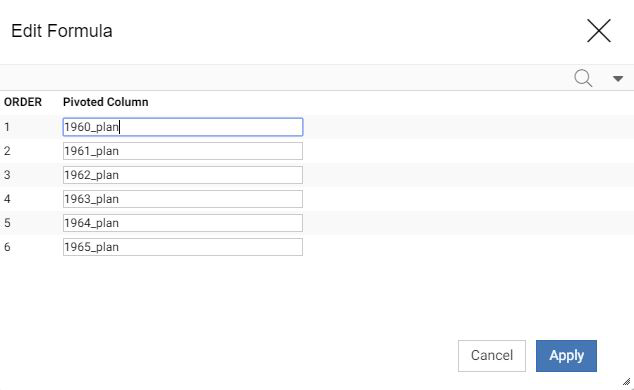
Make sure there are no repetitive alphanumeric values in the Pivoted Column
field. In the example above, delete _plan in each field to show only the year.
9. Click Apply.
An example of the completed configuration for pivoting groups of columns is shown in the following image.
10. Click OK.
The repeating groups of columns now display as rows.
Note: To revert your pivoting changes, right-click the synonym on the Join Editor canvas, and click Remove Pivot.
- Release: 8206
- Category: Connecting to Data
- Product: WebFOCUS Home Page